
convolution 연산은 이미지의 feature를 추출해준다.
filter의 종류에 따라 다른 feature가 추출된다.
진짜로 그런지 실제 이미지를 가지고 convoultion 연산을 하고
그 결과 이미지가 어떻게 나오는지 Tensorflow 1.15 버전으로 확인해보았다.
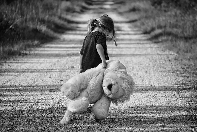
사용한 이미지
코드
사용한 이미지는 3차원이미지이지만 실습을 위해서 channel을 1개만 이용했다.
import numpy as np
import tensorflow as tf
import matplotlib.pyplot as plt
import matplotlib.image as img


ori_img = img.imread('/content/drive/MyDrive/img/girl-teddy.jpg')
print('원본이미지 shape : ', ori_img.shape)

# 입력이미지의 형태
# (1, 429, 640, 3)
input_img = ori_img.reshape((1, )+ ori_img.shape) # 튜플 합으로 shape을 나타냄
# input_img = np.array([ori_img]) # 이렇게 나타내도 같은 결과가 나온다.

print('입력이미지 shape : ',input_img.shape)

# 데이터를 실수로 변환
input_img = input_img.astype(np.float32)

# 차원 변경, slicing
ch1_input_img = input_img[:,:,:,0:1]
print('1차원이미지 shape', ch1_input_img.shape)

# filter의 형태
# (3,3,1,1)
# 윤곽선 필터
weight = np.array([[[[-1]],[[0]],[[1]]],
                   [[[-1]], [[0]],[[1]]],
                   [[[-1]], [[0]], [[1]]]])
print('필터 shape : ', weight.shape)원본이미지 shape : (429, 640, 3)
입력이미지 shape : (1, 429, 640, 3)
1차원이미지 shape (1, 429, 640, 1)
필터 shape : (3, 3, 1, 1)
▶ convolution
stride = 1이고 padding 없이 convolution 연산을 한 번 해주었다.
# stride = 1
# no padding
conv2d = tf.nn.conv2d(ch1_input_img, weight, strides=[1], padding='VALID')

sess = tf.Session()
conv_img = sess.run(conv2d)
print('convolution 이미지 shape : ', conv_img.shape)convolution 이미지 shape : (1, 427, 638, 1)
▶ pooling
pooling_result = tf.nn.max_pool(conv_img,
                                ksize=[1,3,3,1], # 3 x 3 kernel
                                strides=[1,3,3,1], # kernel size와 동일하게
                                padding='VALID')
pool_img = sess.run(pooling_result)
print('pooling 이미지 shape : ', pool_img.shape)pooling 이미지 shape : (1, 142, 212, 1)
pooling을 할 때 stride는 kernel의 사이즈와 똑같이 주어야 한다.
[CNN] Pooling
Pooling, Subsampling CNN과정에서 Convolution Layer를 계속 거치다보면 데이터의 양이 계속적으로 많아진다. 너무 많은 데이터의 양은 학습과정을 방해할 수 있기때문에 데이터의 양을 효율적으로 줄여주
stop-thinking-start-now.tistory.com
이제 단계를 다 마쳤으니 이미지를 하나씩 확인해본다.
images = [ori_img, ch1_input_img.squeeze(), conv_img.squeeze(), pool_img.squeeze()]
titles = ['original image', '1 channel image', 'convolution image', 'pooling image']
fig = plt.figure(figsize=(15,8))
ax = []
for i, img in enumerate(images) :
    ax.append(fig.add_subplot(1,4, i+1))
    ax[i].imshow(img)
    ax[i].set_title(titles[i])

plt.tight_layout()
plt.show()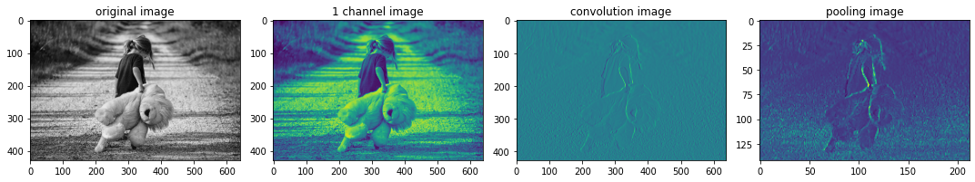
원본 이미지에서 1 채널만 이용했어도 이미지의 특성은 사라지지 않았고,
convolution 연산 후 이미지의 윤곽선 특징이 잘 살아있는 이미지를 얻을 수 있다.
또 pooling으로 이미지의 사이즈는 줄어들었지만 특성은 그대로 가지고 있는 것을 확인할 수 있었다.
▶ activation - ReLu
위의 예시에는 포함되지 않았지만 convolution연산 후에 Activation을 해준다.
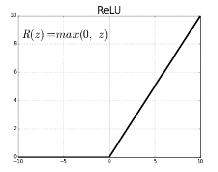
일반적으로 사용하는 활성화함수는 ReLu로,
ReLu는 0이하의 값은 모두 0으로 0이상의 값은 그대로 사용하는 activation function이다.
Sigmoid를 사용할 수도 있지만 Sigmoid를 사용하면 backpropagation,
역전파 과정에서 gradient vanishing현상이 일어나기 때문에 ReLu를 사용한다.
ReLu를 사용하는 의미는 픽셀이 해당 feature를 가지고 있는가 없는가를 판단하는 것이다.
Tensorflow로는 다음과 같이 작성할 수 있다.
relu_ = tf.nn.relu(conv2d_result)
activated_result = sess.run(relu_)'Programming > Tensorflow' 카테고리의 다른 글
| [tensorflow] multi-output model 데이터 입력 : flow_from_dataframe (0) | 2022.07.05 |
|---|---|
| [Tensorflow 1.15 ] Convolution 연산 - Sample Case (2) | 2022.04.14 |
| [Tensorflow] MNIST DNN으로 구현해보기 (0) | 2022.04.12 |
| [Tensorflow] 학습한 모델 저장하기 (0) | 2022.04.07 |
| [Tensorflow] Tensorflow 2.xx with Keras (0) | 2022.04.07 |